Forest fires

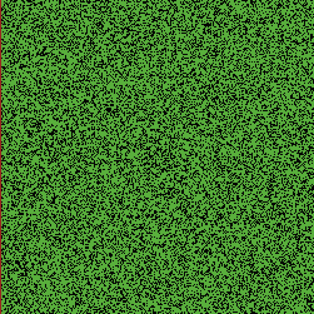
In this article, we will examine a simple model representing the spread of a forest fire. This model has been adapted from an example available on the official NetLogo website. We represent a forest area using green squares for trees and black squares for rocks. The image below illustrates such a forest piece.

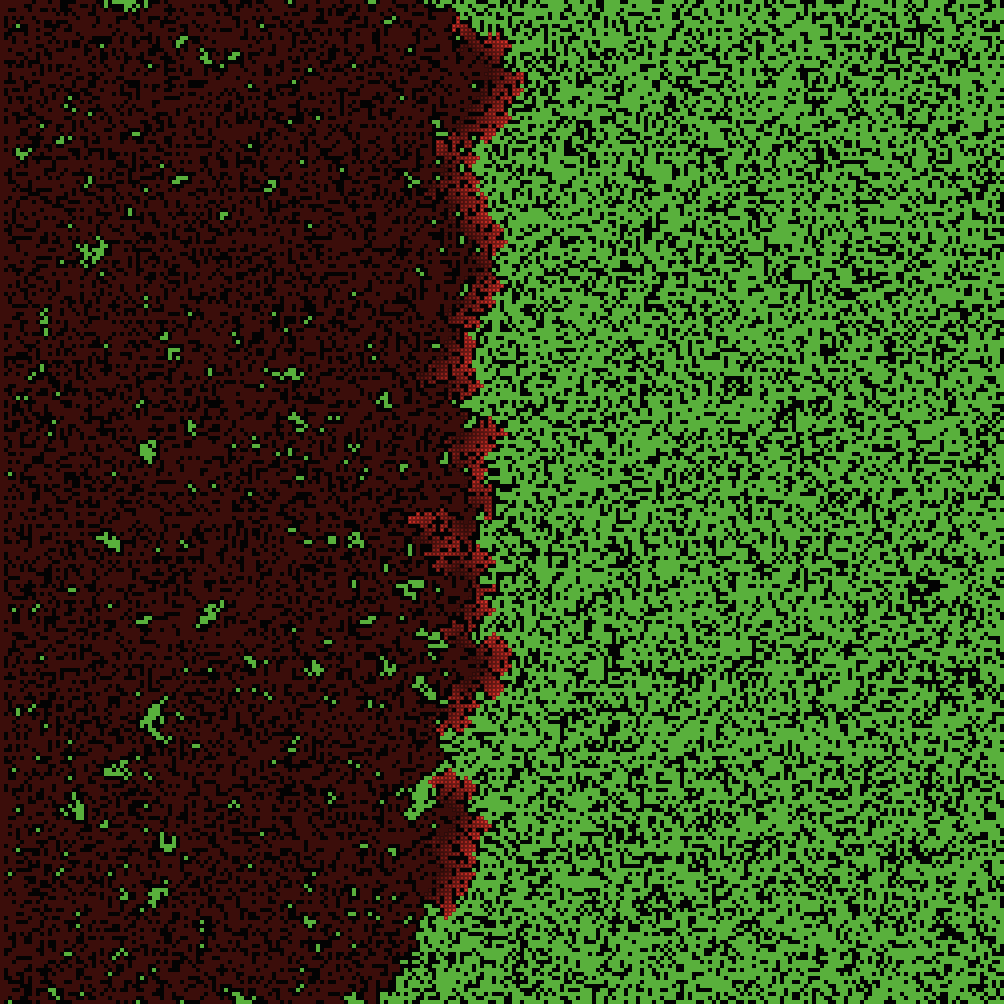
We aim to model the spread of a forest fire. Initially, we ignite a fire on the left side of the forest, represented by red squares. The fire can only consume trees (green squares) and black squares act as barriers preventing the fire from spreading. When a tree is burned, its square turns brown. The image below illustrates an example of fire propagation.

Here, you can launch simulations to see for yourselves how fires propagate. You can choose the initial density of trees (the proportion of green squares among the total number of squares). Then, click on “setup” to initialize the simulation and on “go” to launch it.

You can restart the simulation with a different initial density of trees. Select the initial density of trees, and click again on “Setup” and on “Go”.

We can observe that depending on the tree density (the proportion of green squares), fires may spread more or less. Indeed, for low density, the fire quickly stops. On the opposite, when the density of trees is large enough, the fire propagates to the right side of the forest.

Now, what tree density will you choose to maximize the production of wood without risking that a fire burns most of the forest? Try restarting the simulation (setup) with different densities to maximize the final value of the ‘density of trees still alive.’

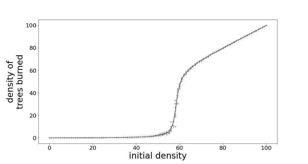
In order to estimate the optimal value, I have repeated the experiment 10 times for every density. On the graph below, each cross represents the final value of one numerical experiment. The line is the average of the different simulations. First, we can observe that the density of trees burned increases with the initial density. This makes sense—the more trees present, the more trees can burn. However, the relationship is not linear; in other words, it is not a straight line. For small densities (lower than 50%), almost no trees burn because the fire cannot propagate. However, at a critical value around 0.59, the fire can propagate to the whole forest, and most trees will burn. This point as been estimated recently by Newman and Ziff. Beyond this point, increasing the density of initial trees will increase the density of burned trees in a similar way, as the fire propagates almost everywhere, and most trees burn.

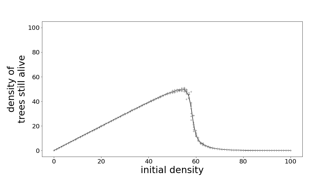
Let’s recall the aim of our model: we want to know what is the optimal density of trees to maximize the number of trees without risking them to burn. Thus, we need to represent the density of trees still alive as a function of the initial density. Now, we can estimate this value around 55%.

You may be wondering if this model can really be used to prevent forest fires. I think this model is too simplistic and relies on hypotheses that are not empirically established. Then, knowing the precise value of the critical point may not be relevant. However, what is more interesting is the qualitative result that the density of burned trees and the initial trees is not linear. More precisely, there is a critical point where the dynamics change.

More importantly, the concept of a ‘critical parameter’ can be applied in many different fields. The theory used here is percolation theory, which is employed in materials science, chemistry, or physics.